The navigation part of the stereo driving system is based on an existing CMU Distributed Architecture for Mobile Navigation (DAMN), which provides a framework within which individual components can be combined into a coherent navigation system [6].
In DAMN, modules communicate using a common set of arcs of constant radii [2][13]. Each module describes its current view of where the vehicle should steer next in terms of votes for a set of arcs. The votes from multiple behaviors are combined by an arbiter which decides on the best command to send to the vehicle controller.
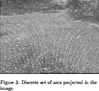
Figure 3 shows the set of arcs used in the current system projected in one of the images. The parameters necessary for projecting the arcs in the image can be computed by a procedure similar to the one used in Section 2.2. The difference is that this procedure uses features tracked over several frames as the vehicle is moving instead of features detected in static images.
The obstacle avoidance module we developed periodically produces recommendations for the best steering directions based on stereo measurements. In other words, this module computes which arcs are safe without attempting to steer the vehicle in a preferred direction. The final steering commands is selected by an arbiter module which is responsible for the arbitration between the different modules involved in a given mission.
The recommendations are encoded in the form of an array of votes for a fixed set of possible arcs of radii
. The votes are encoded as continuous values between -1 and
+1. The semantics of the votes are as follows: If
, the
behavior has determined that the arc of radius
should not be
executed; if
, the behavior has determined that the arc of
radius
is an optimal arc to follow; if
, the
behavior indicates a level of preference for this arc proportional to
.
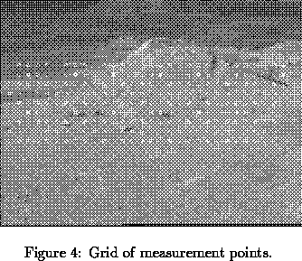
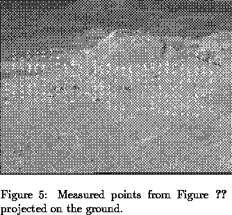
In order to compute these votes, we measure the height and the position on the ground of a few hundred points in the field of view using the algorithms of Section 2.2. Since we know the transformation between the ground plane and the image plane, we select these points on a grid in the image so that they cover a surface on the ground that fits the navigation requirements. The example in Figure 4 shows the grid of measurement points in a typical example and Figure 5 shows their projections on the ground. These points cover an area on the ground ranging between 12 and 32 meters from the robot.
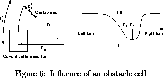
The obstacle
avoidance behavior first computes a vote
for all radii
and all points
(Figure 6). Intuitively,
is the vote that would be assigned to cell
if it were
an obstacle. For reasons of space, we give only a qualitative description of the computation of
. The detail algorithm is described in [2]
and [6].
The computation of is based on three parameters:
, the
distance along the arc after which an obstacle does not matter;
, the
distance along the arc before which an obstacle causes the arc to be removed
from consideration; and
, a coefficient which indicates how fast
increases as function of the lateral distance between the arc and the obstacle
cell. Qualitatively,
decreases as the distance
of the cell along the
arc decreases and is set to 1 (resp -1) if
if greater (resp. lower)
than
(resp.
). Moreover, for cells that do not directly
intersect the arc,
increases with the lateral distance
between
the arc and the cell.
Given a measured point at grid location
, and with relative
height
, the vote for arc
is a function of
and is computed as:
. In this
expression,
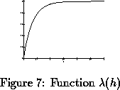
is a function that is small when
is
small, and that converges to 1 as
increases (Figure 7).
With this definition,
is small when the point is close to the
ground plane and becomes close to
, the obstacle value, as the
elevation increases.
The
gain controls the sensitivity of the system to variations in height.
A large value for
causes the system to be sensitive to small variations in
terrain elevation; a small
causes the system to respond only to large objects.
Given now a set of measured points
, the final votes for each arc
are obtained by taking the minimum
values of the
for each measured point.
Using this definition of the votes, we can precompute in a grid
all the for all the arcs and for all the possible cells
in front of the robot.
This speeds up considerably the computation of the final votes.
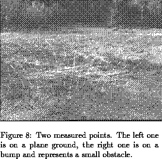
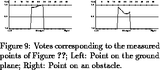
Figure 8 shows two measured points and their influence on the arcs. The first one, on the left, is on the ground plane and is not an obstacle. Its influence on the arcs is shown in Figure 9 on the left. If only one point had been measured, the votes for the arcs on the right would have been slightly higher. (Indeed, the votes for each visible arc are close to 1, and decrease a little for the arcs on the left.) On the contrary, the votes generated by the measure of the second point in the right of the image presented in Figure 9 show clearly that it represents a small obstacle. The values for the votes corresponding to the arcs on the right are much lower than the ones on the left.